Data Build Tool (DBT) – The Emerging Standard For Building SQL-First Data Transformation Pipelines – Part 2

In Part 1 of this series, I went over the high-level introduction to dbt, stood up a small development SQL Server database in Azure, acquired a sample size of Google Analytics data to populate a few tables used in this post and finally installed and configured dbt on a local environment. In this post I’d like to dive deeper into dbt functionality and outline some of its key features that make it an attractive proposition for data transformation and loading part of the ETL/ELT process.

DBT Models

In dbt framework, a model is simply a SELECT SQL statement. When executing dbt run command, dbt will build this model in our data warehouse by wrapping it in a CREATE VIEW AS or CREATE TABLE AS statement. By default dbt is configured to persist those SELECT SQL statements as views, however, this behaviour can be modified to take advantage of other materialization options e.g. table, ephemeral or incremental. Each type of materialization has its advantages and disadvantages and should be evaluated based on a specify use case and scenario. The following image depicts core pros and cons associated with each approach.

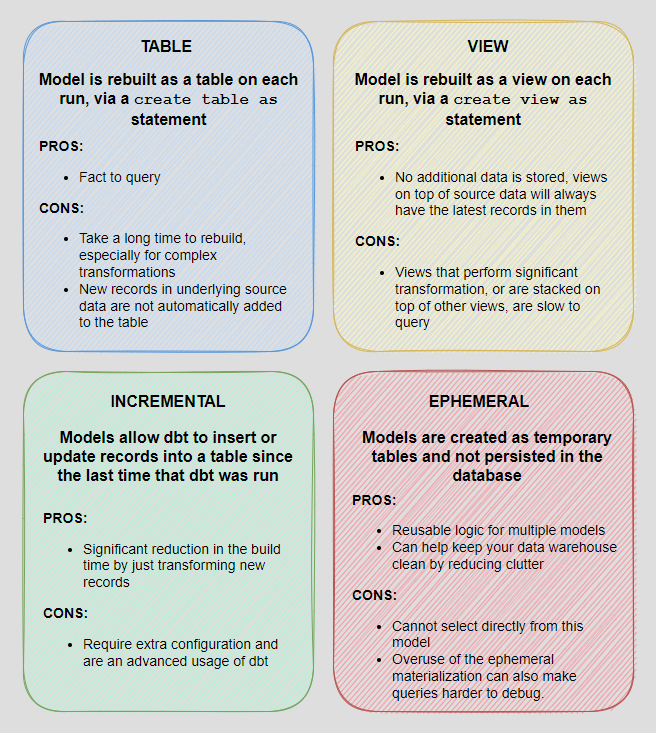
Before we dive headfirst into creating dbt models, first, let’s explore some high-level guiding principles around structuring our project files. The team at dbt recommends organizing your models into at least two different folders – staging and marts. In a simple project, these may be the only models we build; more complex projects may have a number of intermediate models that provide a better logical separation as well as accessories to these models.

• Staging models – the atomic unit of data modeling. Each model bears a one-to-one relationship with the source data table it represents. It has the same granularity, but the columns have been renamed, recast, or standardized into a consistent format
• Marts models – models that represent business processes and entities, abstracted from the data sources that they are based on. Where the work of staging models is limited to cleaning and preparing, fact tables are the product of substantive data transformation: choosing (and reducing) dimensions, date-spinning, executing business logic, and making informed decisions based on business requirements

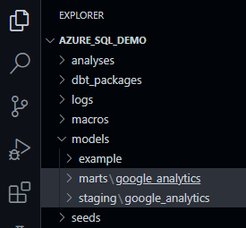Sometimes, mainly due to the level of data complexity or additional security requirements, further logical separation is recommended. In this case ‘Sources’ models layer is introduced before data is loaded into the Staging layer. Sources store schemas and tables in a source-conformed structure (i.e. tables and columns in a structure based on what an API returns), loaded by a third party tool.

Because we often work with multiple data sources, in our Staging and Marts directories, we create one folder per source – in our case, since we’re only working with a single source, we will simply call these google_analytics. Conforming to the dbt minimum standards for project organization and layout i.e. Staging and Marts layers, let’s create the required folders so that the overall structure looks as the one on the left.

At this point we should have everything in place to build our first model based on the table we created in the Azure SQL Server DB in the previous post. Creating simple models is dbt is a straightforward affair and in this case it’s just a SELECT SQL statement. To begin, in our staging\google_analytics folder we create a SQL file, name it after the source table we will be staging and save it with the following two-line statement.

{{ config(materialized='table') }}
SELECT * FROM ga_data

The top line simply tells dbt to materialize the output as a physical table (default is a view) and in doing that select everything from our previously created dbo.ga_data table into a new stg.ga_data table. dbt uses Jinja templating language, making a dbt project an ideal programming environment for SQL. With Jinja, we can do transformations which are not typically possible in SQL, for example, using environment variables or macros to abstract snippets of SQL, which is analogous to functions in most programming languages. Whenever you see a {{ … }}, you’re already using Jinja.

To execute this model, we will simply issue ‘dbt run’ command (here with an optional parameter ‘–select staging’, denoting the name of the model we want to compile) and the output should tell us that we successfully created a staging version of our ga_data table.

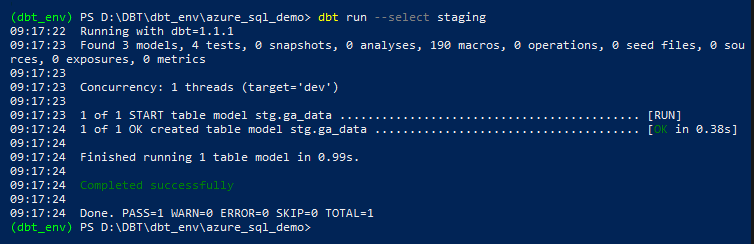
Obviously, in order to build more complete analytics, we need to combine data from across multiple tables and data sources so let’s create another table called ‘ga_geo_ref_data’ containing latitude, longitude and display name values using Geopy Python library. Geopy makes it easy to locate the coordinates of addresses, cities, countries, and landmarks across the globe using third-party geocoders. This will provide us with an additional reference data which we will blend with the core ‘ga_data’ table/model and create a single, overarching dataset containing both: Google Analytics data and reference Geo data used to enrich it.

from pathlib import PureWindowsPath
import pyodbc
import pandas as pd
from geopy.geocoders import Nominatim

_SQL_SERVER_NAME = 'gademosqlserver2022.database.windows.net'
_SQL_DB = 'sourcedb'
_SQL_USERNAME = 'testusername'
_SQL_PASSWORD = 'MyV3ry$trongPa$$word'
_SQL_DRIVER = '{ODBC Driver 18 for SQL Server}'

geolocator = Nominatim(user_agent='testapp')


def enrich_with_geocoding_vals(row, val):
    loc = geolocator.geocode(row, exactly_one=True, timeout=10)
    if val == 'lat':
        if loc is None:
            return -1
        else:
            return loc.raw['lat']
    if val == 'lon':
        if loc is None:
            return -1
        else:
            return loc.raw['lon']
    if val == 'name':
        if loc is None:
            return 'Unknown'
        else:
            return loc.raw['display_name']
    else:
        pass


try:
    with pyodbc.connect('DRIVER='+_SQL_DRIVER+';SERVER='+_SQL_SERVER_NAME+';PORT=1433;DATABASE='+_SQL_DB+';UID='+_SQL_USERNAME+';PWD=' + _SQL_PASSWORD) as conn:
        with conn.cursor() as cursor:
            if not cursor.tables(table='ga_geo_ref_data', tableType='TABLE').fetchone():
                cursor.execute('''CREATE TABLE dbo.ga_geo_ref_data (ID INT IDENTITY (1,1),
                                                            Country NVARCHAR (256),
                                                            City NVARCHAR (256),
                                                            Latitude DECIMAL(12,8),
                                                            Longitude DECIMAL(12,8),
                                                            Display_Name NVARCHAR (1024))''')
            cursor.execute('TRUNCATE TABLE dbo.ga_geo_ref_data;')
            query = "SELECT country, city FROM dbo.ga_data WHERE city <> '' AND country <> '' GROUP BY country, city;"
            df = pd.read_sql(query, conn)
            df['latitude'] = df['city'].apply(
                enrich_with_geocoding_vals, val='lat')
            df['longitude'] = df['city'].apply(
                enrich_with_geocoding_vals, val='lon')
            df['display_name'] = df['city'].apply(
                enrich_with_geocoding_vals, val='name')
            for index, row in df.iterrows():
                cursor.execute('''INSERT INTO dbo.ga_geo_ref_data
                                    (Country,
                                    City,
                                    Latitude,
                                    Longitude,
                                    Display_Name)
                          values (?, ?, ?, ?, ?)''',
                               row[0], row[1], row[2], row[3], row[4])

            cursor.execute('SELECT TOP (1) 1 FROM dbo.ga_geo_ref_data')
            rows = cursor.fetchone()
            if rows:
                print('All Good!')
            else:
                raise ValueError(
                    'No data generated in the source table. Please troubleshoot!'
                )
except pyodbc.Error as ex:
    sqlstate = ex.args[1]
    print(sqlstate)

We will also materialize this table using the same technique we tested before and now we should be in a position to create our first data mart object, combining ga_geo_ref_data and ga_data into a single table.

This involves creating another SQL file, this time in our marts\google_analytics folder, and using the following query to blend these two data sets together.

{{ config(materialized='table') }}

SELECT ga.*, ref_ga.Latitude, ref_ga.Longitude, ref_ga.Display_Name 
FROM {{ ref('ga_data') }} ga
LEFT JOIN {{ ref('ga_geo_ref_data') }} ref_ga
ON ga.country = ref_ga.country 
AND ga.city = ref_ga.city

As with one of the previous queries, we’re using the familiar configuration syntax in the first line but there is also an additional reference configuration applied which uses the most important function in dbt – the ref() function. For building more complex models, ref() function is very handy as it allows us to refer to other models. ref() is, under the hood, actually doing two important things. First, it is interpolating the schema into our model file to allow us to change our deployment schema via configuration. Second, it is using these references between models to automatically build the dependency graph. This will enable dbt to deploy models in the correct order when using ‘dbt run’ command.

If we were to run this model as is, dbt would concatenate our default schema name (as expressed in the profiles.yml file) with the schema we would like to output it into. It’s a default behavior which we need to override using a macro. Therefore, to change the way dbt generates a schema name, we should add a macro named generate_schema_name to the project, where we can then define our own logic. We will place the following bit of code in the macros folder in our solution and define our custom schema name in the dbt_project.yml file as per below

{% macro generate_schema_name(custom_schema_name, node) -%}
    {%- set default_schema = target.schema -%}
    {%- if custom_schema_name is none -%}
        {{ default_schema }}
    {%- else -%}
        {{ custom_schema_name | trim }}
    {%- endif -%}
{%- endmacro %}

name: 'azure_sql_demo'
version: '1.0.0'
config-version: 2

# This setting configures which 'profile' dbt uses for this project.
profile: 'azure_sql_demo'

# These configurations specify where dbt should look for different types of files.
# The 'model-paths' config, for example, states that models in this project can be
# found in the 'models/' directory. You probably won't need to change these!
model-paths: ['models']
analysis-paths: ['analyses']
test-paths: ['tests']
seed-paths: ['seeds']
macro-paths: ['macros']
snapshot-paths: ['snapshots']

target-path: 'target'  # directory which will store compiled SQL files
clean-targets:         # directories to be removed by `dbt clean`
  - 'target'
  - 'dbt_packages'

# Configuring models
# Full documentation: https://docs.getdbt.com/docs/configuring-models
models:
  azure_sql_demo:
    staging:
      +materialized: view
      +schema: stg
    marts:
      +materialized: view
      +schema: mart

With everything in place, we can now save our SQL code into a file called ga_geo.sql and execute dbt to materialize it in a mart schema using ‘dbt run –select marts’ command. On model built completion, our first mart table should be persisted in the database as per the image below (click to enlarge).

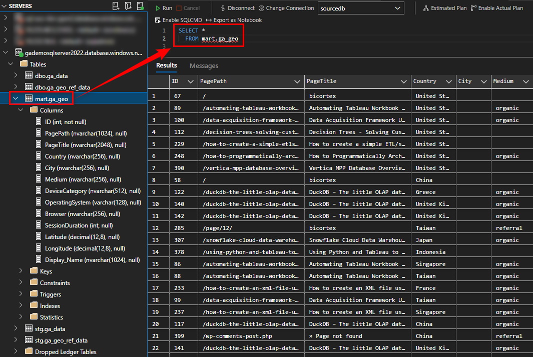
Another great feature of dbt is the ability to create snapshots which is synonymous with the concept of Slowly Changing Dimensions (SCD) in data warehousing. Snapshots implement Type-2 SCD logic, identifying how a row in a table changes over time. If we were to issue an ALTER statement to our ‘ga_data’ table located in the staging schema and add one extra column denoting when the row was created or updated, we could track it’s history using a typical SCD-2 pattern i.e. expiring and watermarking rows which were changed or added using a combination of GUIDs and date attributes.

For this demo let’s execute the following SQL statement to alter our ga_data object, adding a new field called UpdatedAt with a default value of current system timestamp.

ALTER TABLE stg.ga_data
ADD UpdatedAt DATETIME DEFAULT SYSDATETIME()

Once we have our changes in place we can add the following SQL to our solution under the snapshots node and call it ga_data_snapshot.sql.

{% snapshot ga_data_snapshot %}
    {{
        config(
          target_schema = 'staging',
          unique_key = 'ID',
          strategy = 'check',
          check_col = 'all'
        )
    }}
    SELECT * FROM ga_data
{% endsnapshot %}

Next, running ‘dbt snapshot’ command a new table in the staging schema is created and a few additional attributes added to allow for SCD Type-2 tracking (click on image to enlarge).

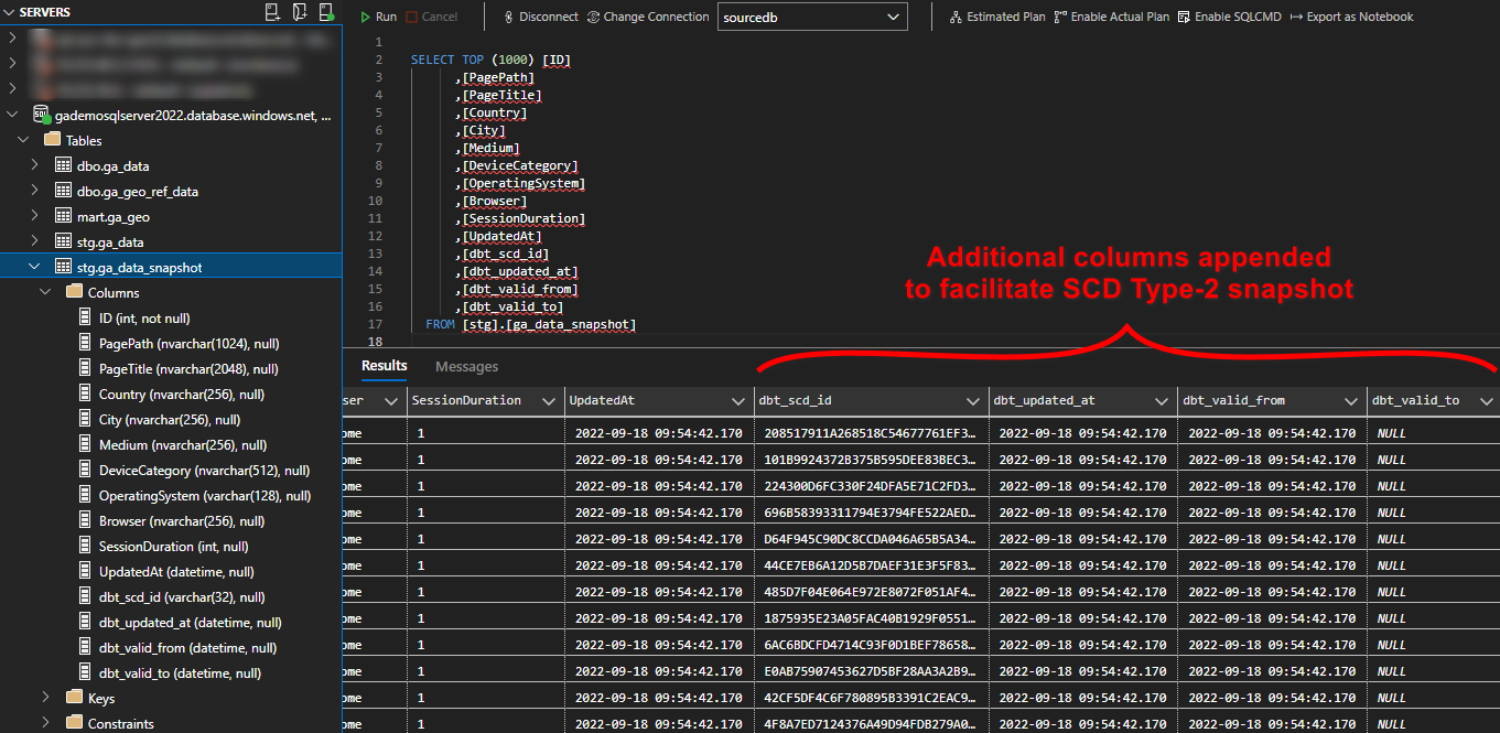
Snapshots are a powerful feature in dbt that facilitate keeping track of our mutable data through time and generally, they’re as simple as creating any other type of model. This allows for very simple implementation of the SCD Type-2 pattern, with no complex MERGE or UPDATE and INSERT (upsert) SQL statements required.

DBT Tests

Testing data solutions has been notoriously difficult and data validation and QA has always been an afterthought. Best case scenario, third party applications had to be used to guarantee data conformance and minimal standards. Worst case, tests were not developed at all and the job of validating the final output fell on analysts or report developers, eyeballing dashboards before pushing them into production. In extreme cases, I even saw customers being delegated to the roles of unsuspected testers, having raising support tickets due to dashboards coming up empty.

In dbt, tests are assertions we make about the models and other resources in our dbt project. When we run dbt test, dbt will tell us if each test in our project passes or fails. There are two ways of defining tests in dbt:

• A singular test is testing in its simplest form: If we can write a SQL query that returns failing rows, we can save that query in a .sql file within our test directory. It’s now a test, and it will be executed by the dbt test command
• A generic test is a parametrized query that accepts arguments. The test query is defined in a special test block (similar to a macro). Once defined, you we reference the generic test by name throughout our .yml files — define it on models, columns, sources, snapshots, and seeds. dbt ships with four generic tests built in: unique, not_null, accepted_values and relationships

In our scenario, we will use generic tests to ensure that:

• The id field on our ga_geo_ref_data is unique and does not contain any NULL values
• The DeviceCategory attribute should only contain a list of accepted values

Test definitions are stored in our staging directory, in a yml file called ‘schema.yml’ and once we issue dbt test command, the following output is generated, denoting all test passed successfully.

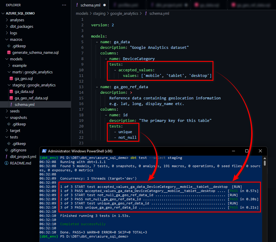
DBT Docs

One of the great features of dbt is the fact we can easily generate a fully self-documenting solution, together with a lineage graph that helps easily navigate through the nodes and understand the hierarchy. dbt provides a way to generate documentation for our dbt project and render it as a website. The documentation includes the following:

• Information about our project: including model code, a DAG of our project, any tests we’ve added to a column, and more
• Information about our data warehouse: including column data types, and table sizes. This information is generated by running queries against the information schema

Running ‘dbt docs generate’ command instructs dbt to compiles all relevant information about our project and warehouse into manifest.json and catalog.json files. Next, executing ‘dbt docs serve’ starts a local web server (http://127.0.0.1:8080) and allows dbt to use these JSON files to generate a local website. We can see a representation of the project structure, a markdown description for a model, and a list of all of the columns (with documentation) in the model. Additionally, we can click the green button in the bottom-right corner of the webpage to expand a ‘mini-map’ of our DAG with, relevant lineage information (click on image to expand).

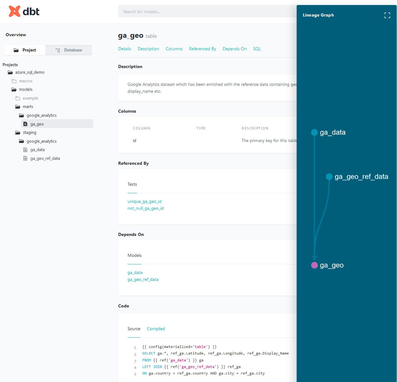
Conclusion

I barely scratched the surface of dbt can do to establish a full-fledged framework for data transformations using SQL and it looks like the company is not resting on its laurels, adding more features and partnering with other vendors. From my limited time with dbt, the key benefits that allow it to stand out in the sea of other tools include:

• Quickly and easily provide clean, transformed data ready for analysis: dbt enables data analysts to custom-write transformations through SQL SELECT statements. There is no need to write boilerplate code. This makes data transformation accessible for analysts that don’t have extensive experience in other programming languages, as the initial learning curve is quite low
• Apply software engineering practices—such as modular code, version control, testing, and continuous integration/continuous deployment (CI/CD)—to analytics code. Continuous integration means less time testing and quicker time to development, especially with dbt Cloud. You don’t need to push an entire repository when there are necessary changes to deploy, but rather just the components that change. You can test all the changes that have been made before deploying your code into production. dbt Cloud also has integration with GitHub for automation of your continuous integration pipelines, so you won’t need to manage your own orchestration, which simplifies the process
• Build reusable and modular code using Jinja. dbt allows you to establish macros and integrate other functions outside of SQL’s capabilities for advanced use cases. Macros in Jinja are pieces of code that can be used multiple times. Instead of starting at the raw data with every analysis, analysts instead build up reusable data models that can be referenced in subsequent work
• Maintain data documentation and definitions within dbt as they build and develop lineage graphs: Data documentation is accessible, easily updated, and allows you to deliver trusted data across the organization. dbt automatically generates documentation around descriptions, models dependencies, model SQL, sources, and tests. dbt creates lineage graphs of the data pipeline, providing transparency and visibility into what the data is describing, how it was produced, as well as how it maps to business logic
• Perform simplified data refreshes within dbt Cloud: There is no need to host an orchestration tool when using dbt Cloud. It includes a feature that provides full autonomy with scheduling production refreshes at whatever cadence the business wants

Obviously, dbt is not a perfect solution and some of its current shortcomings include:

• It covers only the T of ETL, so you will need separate tools to perform Extraction and Load
• It’s SQL based; it might offer less readability compared with tools that have an interactive UI
• Sometimes circumstances necessitate rewriting of macros used at the backend. Overriding this standard behavior of dbt requires knowledge and expertise in handling source code
• Integrations with many (less popular) database engines are missing or handled by community-supported adapters e.g. Microsoft SQL Server, SQLite, MySQL

All in all, I really enjoyed the multitude of features dbt carries in its arsenal and understand why it’s become the favorite horse in the race to dominate minds and hearts of analytics and data engineers. It’s a breath of fresh air, as its main focus is SQL – a novel approach in the landscape dominated by Python and Scala, it runs in the cloud and on-premises and has good external vendors’ support. Additionally, it has some bells and whistles which typically involve integrating with other 3rd party tooling e.g. tests and docs. Finally, at its core, it’s an open-source product and as such, anyone can take it for a spin and start building extensible, modular and reusable ‘plumbing’ for your next project.